

Factor risk model (Barra USE4)#
Use4RiskModel (quantlab.risk.predefined.use4) is a USE4-style factor
risk model built on the BarraStyle exposures (see
Style factors). It follows Menchero, Orr and Wang, The
Barra US Equity Model (USE4), Methodology Notes and Empirical Notes (MSCI,
2011). This page explains the regression and each adjustment, where the
model departs from USE4, and which defaults are MSCI’s published values and
which are quantlab’s own choices. It ends with the model’s numbers on the
Sharadar history and a mean-variance backtest that compares it with
Ledoit-Wolf. Section and equation numbers cite the Methodology Notes as [M]
and the Empirical Notes as [E].
Vocabulary#
A factor return is the return of one factor on one bar: the coefficient of that factor in the bar’s cross-sectional regression of stock returns on exposures.
A specific return is the part of a stock’s return the factors do not explain: its return less its exposures times the factor returns.
The factor covariance
Fis the forecast covariance of the next bar’s factor returns.The specific risk
sof a stock is the forecast volatility of its next specific return.A stock’s forecast covariance is then
X F X' + diag(s^2), withXthe stocks’ exposures.A bias statistic is the standard deviation of returns divided by their forecast volatilities. A calibrated forecast gives 1 (see Bias statistics).
A per-bar data product#
The model is estimated ahead of any backtest, not re-estimated inside it. It writes two stores, one row per bar:
Store |
Variables |
Built from |
|---|---|---|
regression |
|
the exposures and the prices |
estimate |
|
the regression store |
Each store follows the factor lifecycle: compute(start, end) returns
rows, build(start, end) writes them, extend(end) appends the bars after
the recorded range, rewind(end) drops the bars after an earlier end so the
next extend computes them again, and read(start, end) returns a range of
the store. A read outside the range recorded beside the store raises
ValueError. Every row depends only on a bounded window of bars ending at
that bar, so a store built in one go and one built and then extended are
identical, row for row.
Changing an estimate parameter therefore rebuilds only the estimate store.
A store (RiskStore) is written through quantlab.backend.ranged.RangedStore,
the module a factor’s store is written through too: the range is recorded in
<store_path>.range.json, and build, extend and the refusals of read
are that module’s, so a risk store and a factor store say the same thing
about the same problem. A subclass supplies only the rows of a range
(_compute_regression, _compute_estimate). The model declares its two
stores, regression first, with store_uses() (each owns, its RiskStore
the handle); the live day and the daily data update extend what it declares.
from quantlab.risk.config import Use4RiskConfig
from quantlab.risk.predefined.use4 import Use4RiskModel

model = Use4RiskModel(Use4RiskConfig(
    exposures=barra_style,              # a BarraStyle whose store is built
    dataset=prices,                     # adjClose, marketcap and DTB3
    exposure_data_strategy="read",
    risk_free_symbol="DTB3",
    regression_path="risk/use4/regression/regression.zarr",
    estimate_path="risk/use4/estimate/estimate.zarr",
))
model.regression.build("2000-02-03", "2026-10-08")
model.estimate.build("2006-08-10", "2026-10-08")   # after the 1637-bar warm-up
quantlab.risk.base.FactorRiskModel is the contract every factor risk
model meets: the variables of both stores, factor_names,
exposure_names, exposure_matrix and the two warm-ups. It also has
factor_groups(), which gives each factor’s group (country, industry
or style) for a backtest’s factor attribution, and factor_labels(),
each factor’s display name in the backtest report. By default every factor
is a style labelled by its name. Use4RiskModel overrides both from its
config: its industries are named by their Fama-French 48 names and its
styles without the style_ prefix. The USE4 method
lives entirely in Use4RiskModel.
forecast(row, exposures) turns one estimate row and the exposures at
that bar into a FactorRiskForecast, B F B' + diag(D) over the symbols it
covers, with a book’s exposures, variance and x-sigma-rho contributions, and
a factor’s exposures over any symbols (factor_exposure, which the
mean-variance optimiser’s exposure bounds read). It satisfies the
ReturnCovariance protocol a covariance estimator’s estimate meets. It
is the one coverage rule: a symbol with every exposure and a specific risk,
not exposed to a factor without a covariance at the bar (covered_factors).
A portfolio rule reads it through FactorRiskStoreEstimator, which builds
it from the bar’s estimate row and exposures that the decision inputs put in
the context (see
Portfolio construction),
and factor attribution and the random portfolios of the bias statistics
build it too. forecast_window(timestamps) reads, for consecutive bars,
each bar’s factor and specific returns beside the forecast inputs of the
bar before it (estimate row, exposures, risk-free rate, market cap,
estimation universe); factor attribution and the bias statistics read it,
the latter with forecasts_through so the estimate store need only reach
the last forecast bar. require_window(timestamps) checks the stores cover
them, as a backtest does before it simulates.
The regression#
On every bar t, the excess returns of t are regressed on the exposures
of t-1 ([M] §3):
Excess return: adjusted close of
tover adjusted close oft-1, less one, less the risk-free rate oft-1. The rate is FRED’s DTB3, the same seriesBarraStylereads.Factors: a country factor (1 for every stock), one factor per Fama-French 48 industry (1 on the stock’s industry, 0 elsewhere) and the 12 style exposures, 61 factors in all.
Fit: weighted least squares over the estimation universe of
t-1, weighted by the square root of the market cap oft-1, subject to the cap-weighted industry factor returns summing to 0 ([M] eq. 3.3). The constraint removes the collinearity of the country factor with the industries and makes the country factor the cap-weighted market.Diagnostics:
r_squaredis the weighted R-squared1 - sum(w e^2) / sum(w y^2), uncentred because the country factor plays the intercept (our choice).estu_countis the stocks in the fit, andindustry_membersandindustry_excludeddescribe each industry.Thin industries: an industry with fewer than
min_industry_members(5) estimation-universe members on a bar is left out of that bar. It has no factor return that bar, and its members are not in the fit.Outliers: a fitted return more than
return_outlier_sigma(5) robust standard deviations from the cross-sectional median is trimmed to that bound for the fit only. The robust standard deviation is 1.4826 times the median absolute deviation, so a vendor price error cannot move a factor return however large it is.Specific returns: for every stock with all exposures and a return, inside the estimation universe or not, the untrimmed excess return less the fitted factor part. A genuine jump therefore still shows up in specific risk.
The factor covariance#
The factor covariance is built in four steps ([M] §4, Appendix B). Each reads only the last factor returns up to its window.
Exponentially weighted volatilities and correlations ([M] §4.1). The volatilities come from the last 252 factor returns weighted with a half-life of 84 bars, the correlations from the last 1512 with a half-life of 504 (USE4S). A missing factor return (an industry left out of a bar) leaves only that bar out: each correlation uses the bars both factors have.
Newey-West. A variance is multiplied by
C_NW = 1 + 2 sum_l b_l rho_lover 5 lags ([M] eq. 5.2), with Bartlett weightsb_l = 1 - l / (L + 1)and autocorrelationsrho_lweighted with a half-life of 504 over 1512 bars. A correlation is that of the covariance with 2 lags added,G_0 + sum_l b_l (G_l + G_l'). The forecast stays a one-bar forecast: Newey-West turns the variance of a sum of serially correlated one-bar returns into a per-bar variance that scales linearly with the horizon.Eigenfactor risk adjustment ([M] §4.2, Appendix B). The covariance is decomposed into eigenfactors. 1000 factor-return histories are simulated from it, each is estimated with the same windows, half-lives and lags, and the volatility bias of each simulated eigenfactor is measured. Each eigenvariance is then multiplied by the square of its bias, the simulated adjustment of [M] eq. B7. Setting
eigen_scaleuses the scaled adjustment of eq. B8 instead. The draws of a bar are seeded fromeigen_seedand the bar’s timestamp, so a row does not depend on how the store is split betweenbuildandextend.Volatility regime adjustment ([M] §4.3). On each bar, the cross-sectional bias statistic of the factor returns against the forecasts of the bar before is measured. The whole matrix is multiplied by
lambda_F^2, the exponentially weighted mean square of those bias statistics over the last 126 bars with a half-life of 42. The correlations do not move.lambda_Fis stored asfactor_volatility_multiplier.
The specific risk#
Each stock’s specific risk is built in four steps ([M] §5):
Time series ([M] §5.1): the exponentially weighted volatility of its last 252 specific returns, half-life 84, with no Newey-West adjustment by default (see Defaults).
Structural model ([M] eqs. 5.3-5.5). On each bar the log time-series volatility of every stock with a time series is regressed on its exposures and its history length,
log(1 + h / 252)withhits specific returns in the last 756 bars. A stock’s structural volatility isE_0times the exponential of its fitted value,E_0the smearing estimate: the mean ofexp(residual)over the fitted stocks. With the defaultstructural_model="fill", a stock without a time-series value (fewer than 21 returns in the window, a new listing for example) gets its structural value, and every other stock keeps its time series."blend"is USE4’sgamma * time series + (1 - gamma) * structural.Bayesian shrinkage ([M] §5.2, eqs. 5.6-5.9) toward the cap-weighted mean of the stock’s size decile, with intensity
q |s - m| / (d + q |s - m|),q = 0.1. On the Sharadar history a largerqflattened the 21-bar bias statistics across forecast-volatility deciles but worsened the one-bar ones and the random active portfolios’, so USE4’s value stands.Volatility regime adjustment ([M] §5.3): times
lambda_S, the same construction aslambda_Fover the cap-weighted cross-sectional bias statistics of the estimation universe’s specific returns. It is stored asspecific_volatility_multiplier.
Every stock with exposures at the bar has a specific risk once enough stocks are fitted.
Deviations from USE4#
The data quantlab has, and what MSCI does not publish, force some departures:
Factors. The industries are the point-in-time Fama-French 48 from SIC, not GICS, and a stock has one industry rather than several weights. The styles have the deviations of Style factors (no analyst forecasts).
Estimation universe. The 3000 largest stocks by market cap, not the MSCI USA IMI.
Missing factor returns. Correlations use the pairwise-available bars, where USE4 uses the EM algorithm. A pairwise estimate need not be positive semi-definite; the eigenfactor adjustment sets negative eigenvalues to 0.
Windows. USE4 publishes half-lives but not window lengths. Every window here is three half-lives, so a row reads a bounded window and a build equals a build then an extend.
Newey-West. USE4 publishes the lags, not the weights; these are Bartlett’s. USE4 publishes no separate half-life for the factor volatilities’ autocorrelations; weighting them with the volatilities’ 84 measured worse on the Sharadar history (bias statistics over 1- and 21-bar returns), so they use 504. The specific volatilities have no Newey-West adjustment by default: USE4’s published 5 lags with a half-life of 252 also measured worse.
Eigenfactor simulations. USE4 publishes no simulation count or history length: 1000 simulations, each as long as the longest window the covariance reads.
Volatility regime adjustment. The factor bias statistic is the root mean square over the factors with both a forecast and a return, where USE4 divides by every factor. The specific one is weighted by the market caps of the bar before, over its estimation universe; USE4 names no bar or universe.
Structural model. USE4 fits the well-behaved stocks (blending coefficient 1) on their exposures alone, and blends every stock. The default fills only the stocks without a time series, mostly new listings, since blending worsened the specific bias statistics on the Sharadar history. USE4’s structural values ran low for those stocks: their 21-bar bias statistic was 1.36 with outcomes of more than 100% in one bar left out. Three changes bring it to 1.09:
fit on every stock with a time series;
a history-length regressor, the main gain;
E_0estimated each bar by smearing (Duan, 1983), where replications use a fixed 1.05.
With the other two changes, a fixed 1.05 in place of smearing gives 1.10. The blending coefficient’s parameters (60, 120, 10) are not published; these are the values third-party replications of the Barra models use.
Defaults#
Every parameter is a field of Use4RiskConfig. USE4L, the long-horizon
model, is volatility_half_life=252, specific_half_life=252,
vra_half_life=168 and windows of three half-lives.
Field |
Default |
Source |
|---|---|---|
|
12 styles, FF48, yes |
USE4 structure; FF48 ours |
|
|
USE4 ([M] §3) |
|
5 |
ours |
|
5 |
ours |
|
84, 252 |
USE4S half-life; window ours |
|
504, 1512 |
USE4S half-life; window ours |
|
5, 2 |
USE4S |
|
504, 1512 |
ours (USE4: the volatility half-life) |
|
1000, 0 |
ours |
|
|
USE4; eq. B8’s |
|
15 |
USE4 (eq. B8) |
|
42, 126 |
USE4S half-life; window ours |
|
84, 252 |
USE4S half-life; window ours |
|
0 |
ours (USE4: 5) |
|
252, 756 |
USE4 half-life; window ours |
|
|
ours (USE4: blend) |
|
|
ours (USE4: blending coefficient 1) |
|
|
ours (replications: 1.05) |
|
756 |
ours (USE4: none) |
|
60, 120, 10 |
third-party replications |
|
0.1, 10 |
USE4 |
|
21 |
ours |
The estimate store’s warm-up is the longest window less one bar plus the regime adjustment’s window: 1511 + 126 = 1637 regression bars.
Bias statistics#
quantlab.risk.bias.bias_statistics(realized, forecast, window) follows
[M] Appendix A. For each portfolio, the standardized outcome is the
realized return divided by its forecast volatility, and the bias statistic
is the standard deviation of those outcomes. For normal returns and a
right forecast, 95% of bias statistics over T outcomes fall within 1 +/- sqrt(2/T). Above the band the model underpredicts risk, below it
overpredicts. With window it also returns the rolling bias statistic and,
across portfolios, its mean, 5th and 95th percentiles and the mean
absolute deviation from 1 (MRAD).
risk_model_bias_statistics(model, start, end, horizon=h) reads the
outcomes and forecasts straight from a model’s stores, with no backtest,
for four groups of portfolios: each pure factor, each eigenfactor of the
forecast covariance, each stock’s specific return, and 100 random active
portfolios of 500 estimation-universe stocks against the cap-weighted
universe ([E] §5). Over h bars the outcome is the sum of the next h
bars’ returns and the forecast sqrt(h) times the one-bar one, so a
horizon longer than one bar tests the Newey-West adjustment. USE4 tests
monthly (h = 21).
On real data#
examples/sharadar_us_equity/risk_model.py on the training server, on the
2026-10-05 Sharadar pull, the exposures of barra_style.py and FRED’s
DTB3, with every default. The figures and numbers below come from the
example before it read its prices through BadPrintMaskedDataset.
The last subsection gives the bias statistics with bad prints masked.
Size and cost. The regression store covers 6,475 bars (2001-01-03 to 2026-10-02) of 14,772 permatickers and is 256 MB. It builds in 2.6 minutes. The estimate store covers 4,837 bars (2007-07-13 to 2026-10-02, after the 1637-bar warm-up) of 12,144 permatickers and is 268 MB. It builds in 19.5 minutes in 32 processes, most of it the eigenfactor simulations. The bias statistics of both horizons take 2.6 minutes more.
Regression. The fit has a median of 2,998 stocks per bar. The uncentred weighted R-squared has a mean of 0.34 and a median of 0.30. Nine FF48 codes (1, 3, 4, 5, 16, 20, 25, 26 and 27) are left out on every bar, so 52 of the 61 factors have returns; Coal (29) is left out on 4.6% of the bars. The country factor’s annualized volatility is 19.2% and its lag-1 autocorrelation is -0.08.
Forecasts on 2024-06-28. The country factor’s forecast volatility is 10.0% a year. The styles range from 1.3% (Growth) to 6.7% (Beta), with Momentum at 5.1%. 5,264 stocks have a specific risk, with a median of 40.7% a year.
Volatility regime multipliers.
lambda_Fhas a mean of 0.998, a peak of 1.70 on 2020-03-26 and a low of 0.64 on 2009-12-31.lambda_Shas a mean of 1.047 and a peak of 1.70 on the same day.
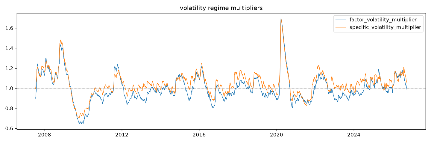
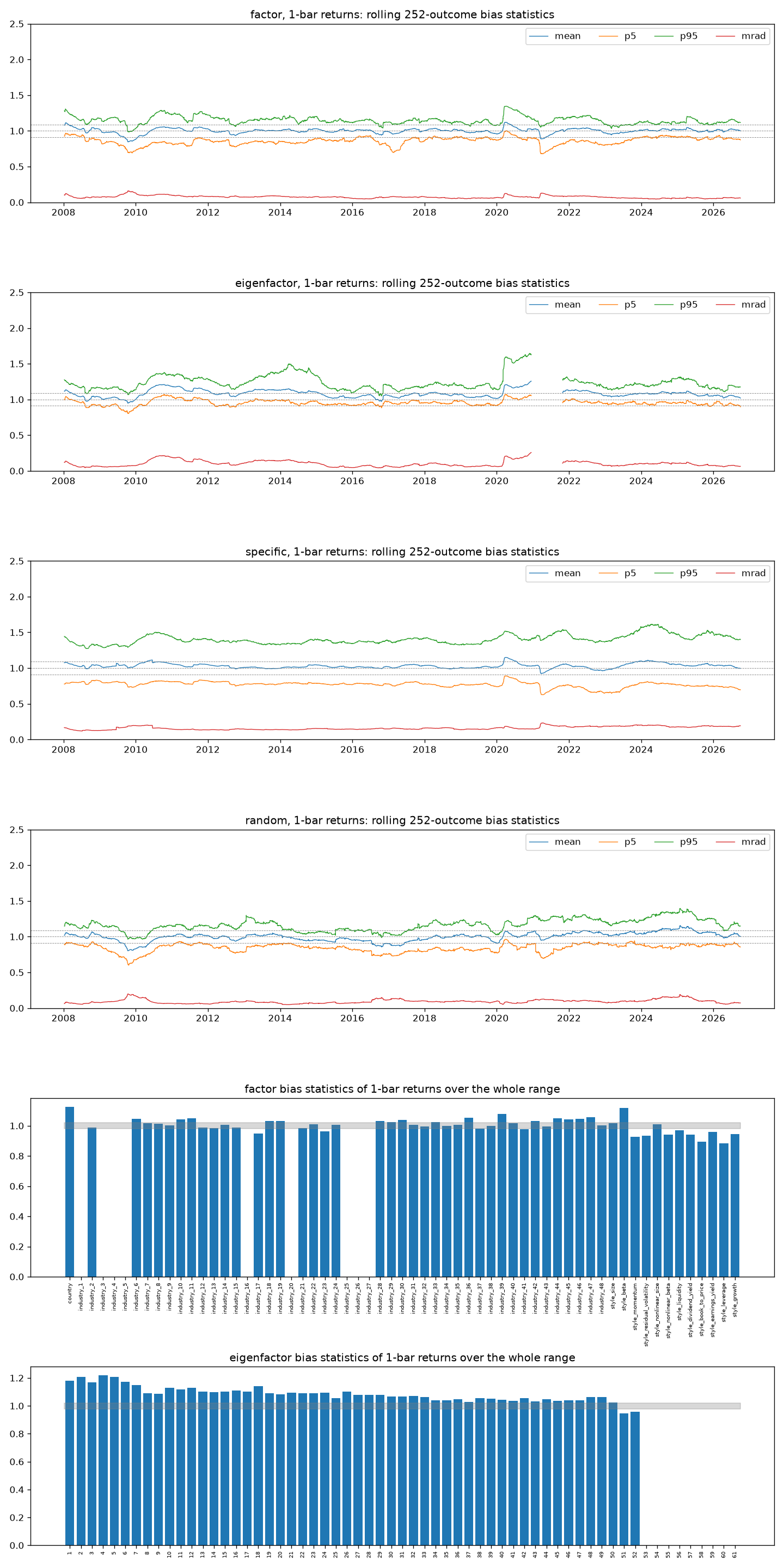
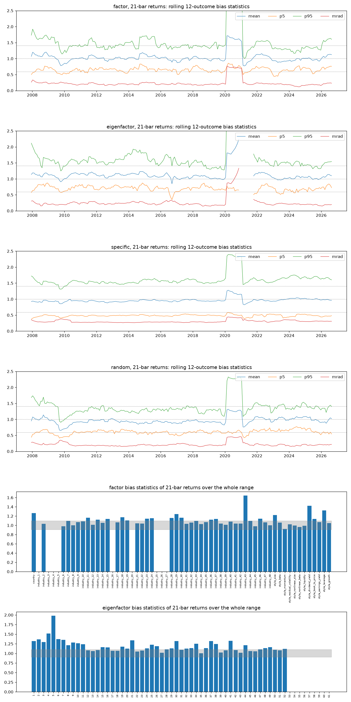
Bias statistics, 2007-07-13 to 2026-10-02 (risk_model_bias_statistics).
A specific return counts only for a stock with at least a year of outcomes.
“In band” is the share of portfolios whose bias statistic is within 1 +/- sqrt(2/T). Over one bar T is about 4,800 and the band is +/-0.02, so a
small bias already falls outside it. MRAD is the mean over time of the
rolling one-year mean absolute deviation from 1.
Group |
Portfolios |
1 bar: mean |
median |
in band |
MRAD |
21 bars: mean |
median |
in band |
MRAD |
|---|---|---|---|---|---|---|---|---|---|
Factors |
52 |
1.004 |
1.006 |
42% |
0.074 |
1.099 |
1.068 |
58% |
0.234 |
Eigenfactors |
52 |
1.084 |
1.078 |
0% |
0.101 |
1.185 |
1.135 |
35% |
0.260 |
Specific |
10,584 |
1.106 |
1.026 |
28% |
0.160 |
1.057 |
0.987 |
57% |
0.303 |
Random active |
100 |
1.003 |
1.005 |
26% |
0.093 |
1.003 |
1.007 |
68% |
0.214 |
The random active portfolios, the closest to what a portfolio rule holds, are calibrated at both horizons: 1.003 on average.
The country factor is underpredicted: 1.126 over one bar and 1.263 over 21. Over one bar Beta is 1.119; most other styles are slightly overpredicted, Leverage the most at 0.882.
The eigenfactors are still underpredicted after the adjustment, the lowest-variance ones the most (about 1.2 for the first six over one bar).
Specific risk is right for the median stock (1.026 over one bar). The mean, 1.106, is pulled up by a tail of stocks whose risk is underpredicted. Pooled by forecast-volatility decile, the top decile looks heavily underpredicted (about 2.5 over one bar and 3.6 over 21). Ten outcomes outside the estimation universe make up most of it: one-bar bad prints such as a close of $0.01 between two of $7 to $9, and real micro-cap jumps. Within the estimation universe, priced at $5 or more, the top decile is overpredicted (about 0.8 at both horizons), as in USE4.
With bad prints masked. This is the example as it stands. The
exposures and the risk model read their prices through
BadPrintMaskedDataset, which flags 535 bars of 321 permatickers.
Group |
1 bar: mean |
median |
in band |
MRAD |
21 bars: mean |
median |
in band |
MRAD |
|---|---|---|---|---|---|---|---|---|
Factors |
1.004 |
1.006 |
40% |
0.075 |
1.099 |
1.069 |
58% |
0.234 |
Eigenfactors |
1.084 |
1.076 |
0% |
0.101 |
1.184 |
1.136 |
31% |
0.257 |
Specific |
1.092 |
1.026 |
28% |
0.156 |
1.036 |
0.985 |
57% |
0.296 |
Random active |
1.005 |
1.009 |
23% |
0.092 |
1.004 |
1.007 |
68% |
0.213 |
Specific risk. The mean bias falls from 1.106 to 1.092 over one bar and from 1.057 to 1.036 over 21. The pooled bias of the top forecast-volatility decile falls from about 2.5 to 1.26 over one bar, and from 3.6 to 1.10 over 21. Within the estimation universe that decile goes from 2.69 (one bad print) to 0.88 over one bar.
What is left of the tail. It is mostly real jumps the rule keeps by design, such as TPST on 2023-10-11 and ORBS on 2025-09-08, and moves after halts longer than the rule’s lookback.
Factors and random portfolios barely move; the regression’s outlier trimming had already kept the bad prints out of the factor returns.
Mean-variance with Ledoit-Wolf and with the factor model#
examples/sharadar_us_equity/sp500_xgb_mvo.py backtests one return model
twice over 2020-2024 on the point-in-time S&P 500. The model is XGBoost on
Alpha101 and Alpha158, predicting the 5-bar return and trained on
2012-2019. Both backtests use the same MeanVarianceOptimizer (Grinold
expected return with ic=0.02, risk aversion 10, turnover penalty 0.001,
2% weight cap, long only, the top 200 predictions as candidates,
rebalanced every 5 bars, fees and slippage of 5 bp each). Only the
covariance differs: LedoitWolfEstimator over 126 one-bar returns, or
FactorRiskStoreEstimator on the estimate store above. Neither backtest
failed a rebalance. Both backtests also pass Use4RiskModel as their
risk_model and attribute their holdings to its factors (see below). On
the training server the factor-model backtest took 5.5 minutes, most of it
computing BarraStyle over the window (measured when the backtest still
computed the exposures instead of reading their store), and the Ledoit-Wolf one 3.1
minutes; the whole script takes 11 minutes.
Ledoit-Wolf |
USE4 factor model |
|
|---|---|---|
Total return |
42.5% |
34.3% |
Annualized return |
7.4% |
6.1% |
Annualized volatility (daily) |
15.9% |
16.0% |
Sharpe ratio |
0.53 |
0.45 |
Max drawdown |
31.9% |
29.7% |
Annualized turnover |
727% |
685% |
Beta to SPY |
0.65 |
0.64 |
Tracking error to SPY |
10.8% |
11.4% |
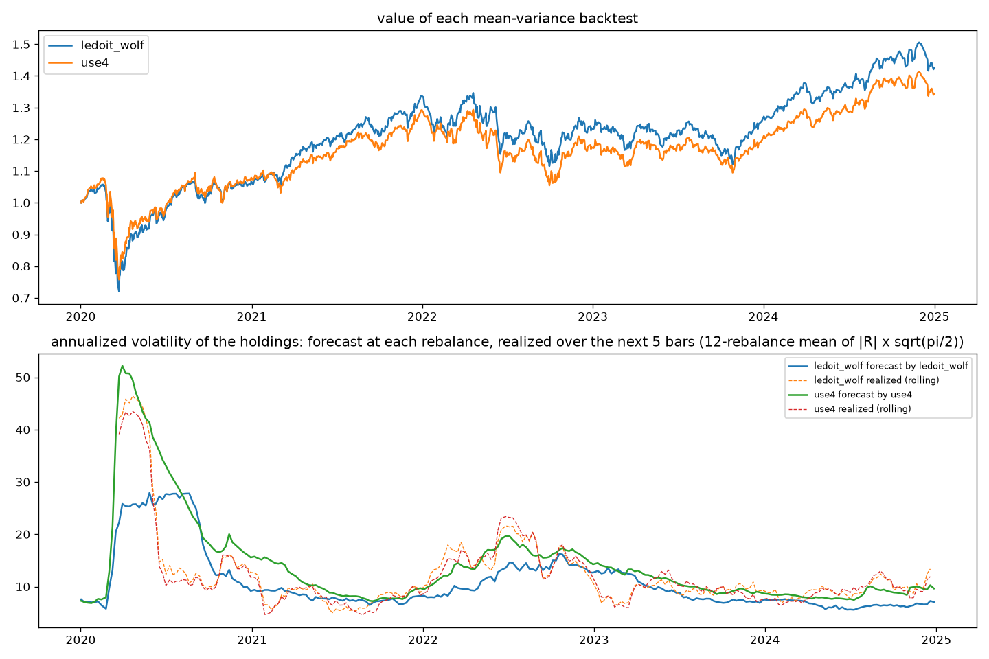
SPY returned 96.8% (14.5% a year, 21.0% volatility) over the same window. The return model is weak, and one five-year path of one model does not separate the two covariances on return.
Risk does separate them. On each of the 251 rebalance bars, each risk
model forecasts the volatility of the holdings over the next 5 bars, and
the forecast is compared with the return the holdings made
(bias_statistics; band +/-0.089):
Holdings of |
Realized volatility |
Ledoit-Wolf forecast |
bias |
USE4 forecast |
bias |
|---|---|---|---|---|---|
Ledoit-Wolf backtest |
15.6% |
10.9% |
1.435 |
15.1% |
1.006 |
USE4 backtest |
14.7% |
12.4% |
1.225 |
14.2% |
1.029 |
Ledoit-Wolf underpredicts the risk of the portfolio it chose by 44%. The optimizer puts weight where the sample covariance happens to be low, so the estimation error lands in the portfolio. Its half-year window also lags a change of regime: in March 2020 it forecast about 25% while the holdings realized over 40%. The factor model forecasts both portfolios within the band, including the one it did not choose.
The factor attribution of the two backtests (the factor_attribution
block of each run’s metrics, 2020-2024, annualized log growth; see
Backtesting)
says where the return came from. The terms add up to each run’s log NAV
on every bar (largest gap 5e-16), and the model covers at least 98% of the
held weight on every bar:
Ledoit-Wolf |
USE4 factor model |
|
|---|---|---|
Country |
9.7% |
9.7% |
Industry |
-0.5% |
-1.0% |
Style |
-4.3% |
-4.8% |
Specific |
0.1% |
-0.1% |
Risk-free |
2.5% |
2.5% |
Trading |
-0.4% |
-0.4% |
Total |
7.1% |
5.9% |
Ex-ante volatility (factor / specific) |
15.1% (14.8% / 3.1%) |
14.2% (13.9% / 2.7%) |
Ex-post volatility |
15.9% |
16.0% |
Both books earned the market and lost on their style exposures. The specific return, the part the return model should add, is about zero, in line with a weak model. The 1.2-point gap in total return between the two is mostly style and industry, not stock selection.