Backtesting#

A backtest replays a strategy over historical prices. The backtester is the last stage of the pipeline: it takes a trained model and a price dataset, turns the model’s predictions into target weights with a portfolio construction rule, simulates trading those weights with vectorbt, and writes a run directory with the weights, the equity curve, the metrics, an HTML report and the recipe that rebuilds the run.

The classes involved are:

BaseBacktester: the steps that do not depend on a simulation engine (dates, warm-up, the in-sample split, metrics, persistence).
VectorBtBacktester: the simulation.
USEquityCrossectionSelectStockVectorBt: the US-equity cross-sectional stock-selection backtester, configured with a CrossSectionBacktestConfig. Its constructor field holds the portfolio rule.
WeightsVectorBt: backtests given weights on any market, without a model; quantlab.api.backtest() runs it.
BacktestRun: reads a run directory back.

examples/backtest.py is a runnable companion on synthetic data that needs no credentials or network access and runs in under a minute:

uv run python examples/backtest.py

Setup#

The sessions on this page use a synthetic setup: six symbols, one factor, one label and a model head with nothing to fit, whose score is the past one-bar return. The label is the factor open_ret_1 wrapped in Forward with span=1 and the default delay=1: its value at bar t is the open-to-open return from t+1 to t+2. The last symbol, FFF, stops trading inside the window. Save the module below as demo_parts.py and run the sessions from the repository root with uv run python. On macOS, set OMP_NUM_THREADS=1 before torch or xgboost is imported in the same process.

demo_parts.py

"""Synthetic prices, a factor, a label and a model with nothing to fit."""
import dataclasses
from pathlib import Path

import numpy as np
import pandas as pd
import polars as pl
import xarray as xr

from quantlab.model.config import ModelConfig
from quantlab.factor.config import PolarsFactorConfig
from quantlab.label.config import ForwardConfig
from quantlab.dataset.config import DatasetConfig
from quantlab.factor.polars import FactorPolars
from quantlab.model.library_model import LibraryModel
from quantlab.dataset.stock import StockDataset
from quantlab.label.forward import Forward

SYMBOLS = ["AAA", "BBB", "CCC", "DDD", "EEE", "FFF"]


def write_price_store(root, n_bars=60, delist=None):
    """Daily adjusted prices in Zarr; delist={"FFF": 36} ends FFF at bar 36."""
    root.mkdir(parents=True, exist_ok=True)
    rng = np.random.default_rng(0)
    shape = (n_bars, len(SYMBOLS))
    close = 50 * np.exp(np.cumsum(rng.normal(0, 0.02, shape), axis=0))
    open_ = np.vstack([close[:1], close[:-1]]) * np.exp(rng.normal(0, 0.01, shape))
    for symbol, bar in (delist or {}).items():
        close[bar:, SYMBOLS.index(symbol)] = np.nan
        open_[bar:, SYMBOLS.index(symbol)] = np.nan
    dims = ["timestamp", "symbol"]
    xr.Dataset(
        {"adjOpen": (dims, open_), "adjClose": (dims, close)},
        coords={"timestamp": pd.bdate_range("2024-01-01", periods=n_bars), "symbol": SYMBOLS},
    ).to_zarr(root / "prices.zarr", mode="w")
    return DatasetConfig(
        raw_data_dir_path=str(root / "raw"), zarr_file_path=str(root / "prices.zarr"),
        market="us_equity", frequency="1d",
    )


def prices_of(cfg):
    return StockDataset(dataclasses.replace(cfg))


class PastReturn(FactorPolars):
    """Feature past_ret_1: the one-bar close-to-close return."""

    def _get_factor_lazyframe(self, lf):
        c = pl.col("adjClose")
        return (lf.sort(["symbol", "timestamp"])
                .with_columns((c / c.shift(1).over("symbol") - 1).alias("past_ret_1"))
                .select(["timestamp", "symbol", "past_ret_1"]))


class OpenReturn(FactorPolars):
    """open_ret_1: the one-bar open-to-open return, using bars up to t only."""

    def _get_factor_lazyframe(self, lf):
        o = pl.col("adjOpen")
        return (lf.sort(["symbol", "timestamp"])
                .with_columns((o / o.shift(1).over("symbol") - 1).alias("open_ret_1"))
                .select(["timestamp", "symbol", "open_ret_1"]))


class MomentumHead(LibraryModel):
    """Predicts its first feature, so the score is the past return."""

    def _init_model(self, num_features, num_labels, hyperparameters):
        return {"num_labels": num_labels}

    def _fit_model(self, train_rows, val_rows):
        pass

    def _forward(self, x):
        return np.repeat(x[..., :1], self.model["num_labels"], axis=-1)


def make_label(cfg, delay=1):
    """Label open_ret_1 at t: the open-to-open return from t+delay to t+delay+1."""
    factor = OpenReturn(PolarsFactorConfig(warmup_bars=1, dataset=prices_of(cfg)))
    return Forward(ForwardConfig(factor=factor, span=1, delay=delay))


def make_model(root, cfg, days, train_end=39, delay=1):
    day = lambda i: str(days[i].date())
    factor = PastReturn(PolarsFactorConfig(warmup_bars=5, dataset=prices_of(cfg)))
    return MomentumHead(ModelConfig(
        factors=[factor], labels=[make_label(cfg, delay)], model_save_dir=str(root / "models"),
        factor_data_strategy="cal", label_data_strategy="cal", val_size=0.0,
        start_date=day(0), end_date=day(len(days) - 1),
        train_start=day(0), train_end=day(train_end),
        test_start=day(train_end + 1), test_end=day(len(days) - 1),
    ))


def train_checkpoint(model):
    model.collect()
    return model.train()


def train_cv_project(model, train_periods):
    model.collect()
    return model.train_cv(train_periods=train_periods).path

A first run#

run() backtests one model over the window start_date to end_date:

It checks every label’s delay against the engine’s fill delay (see Execution timing).
It loads the checkpoint (model_mode="load") or trains the model on its own configured dates first (model_mode="train").
It asks every factor for the window by date range and lets the model predict a panel of scores on (timestamp, symbol).
The portfolio rule turns the scores into target weights on the rebalance bars.
The weights are simulated, metrics computed for the whole window and for its in-sample and out-of-sample parts, and everything is written to a new run directory under output_dir.

The first session trains a checkpoint and backtests a rule that holds the two highest-scoring symbols, rebalancing every five bars. Log lines go to stderr and are not shown.

>>> import dataclasses, tempfile
>>> from pathlib import Path
>>> import pandas as pd
>>> import xarray as xr
>>> from demo_parts import *
>>> from quantlab.backtest.predefined.us_equity import USEquityCrossectionSelectStockVectorBt
>>> from quantlab.backtest.config import CrossSectionBacktestConfig
>>> from quantlab.portfolio.config import TopNConfig
>>> from quantlab.portfolio.predefined.top_n import TopNConstructor
>>> root = Path(tempfile.mkdtemp())
>>> cfg = write_price_store(root, delist={"FFF": 36})
>>> days = pd.bdate_range("2024-01-01", periods=60)
>>> checkpoint = train_checkpoint(make_model(root / "train", cfg, days))
>>> backtester = USEquityCrossectionSelectStockVectorBt(CrossSectionBacktestConfig(
...     price_dataset=prices_of(cfg),
...     model=make_model(root / "backtest", cfg, days),
...     model_mode="load",
...     checkpoint=str(checkpoint),
...     start_date="2024-02-12",
...     end_date="2024-03-22",
...     output_dir=str(root / "runs"),
...     rebalance_periods=5,
...     constructor=TopNConstructor(TopNConfig(direction="long_only", top_n=2)),
... ))
>>> result = backtester.run()
>>> from quantlab.runs.backtest_run import BacktestRun
>>> run = BacktestRun.open(result.run_dir)
>>> run.kind, run.window, run.rebalance_periods
('run', ('2024-02-12', '2024-03-22'), 5)

In load mode the model must still be configured with the same factors and labels, because the backtester recomputes the features; the checkpoint supplies only the fitted parameters. The config is validated when the backtester is built, before any data is read.

With model_mode="train" the model is trained on its own dates and checkpoint is not needed; the window never changes the training dates. The checkpoint is recorded in metrics["trained_checkpoint"], and its unit is the run’s trained_run(). This session also switches to a long-short book with one name per side:

>>> trained = USEquityCrossectionSelectStockVectorBt(dataclasses.replace(
...     backtester.config, model=make_model(root / "train_mode", cfg, days),
...     model_mode="train", checkpoint=None,
...     constructor=TopNConstructor(TopNConfig(direction="long_short", top_n=1)),
... )).run()
>>> Path(trained.metrics["trained_checkpoint"]).name
'MomentumHead_total.joblib'
>>> BacktestRun.open(trained.run_dir).trained_run().checkpoint == Path(trained.metrics["trained_checkpoint"])
True
>>> trained.weights["weight"].to_pandas().iloc[0]
symbol
AAA    0.0
BBB   -0.5
CCC    0.5
DDD    0.0
EEE    0.0
FFF    0.0
Name: 2024-02-12 00:00:00, dtype: float64

Target weights and rebalancing#

Whatever rule produces them, the engine simulates target weights: a weight variable on (timestamp, symbol). A finite weight is the fraction of portfolio value the symbol should be worth after the order fills, negative for a short; a NaN keeps the symbol’s holding untraded. An all-NaN row is a bar without a rebalance. The gross exposure of a row (the sum of absolute weights) is at most 1, so the portfolio is never leveraged. The shipped rules give every symbol a finite weight on a rebalance bar, 0.0 for one not selected; a rebalance with nothing to buy is all zeros, not all NaN.

>>> result.weights["weight"].to_pandas().iloc[:7].round(2)
symbol      AAA  BBB  CCC  DDD  EEE  FFF
timestamp                               
2024-02-12  0.0  0.0  0.5  0.0  0.0  0.5
2024-02-13  NaN  NaN  NaN  NaN  NaN  NaN
2024-02-14  NaN  NaN  NaN  NaN  NaN  NaN
2024-02-15  NaN  NaN  NaN  NaN  NaN  NaN
2024-02-16  NaN  NaN  NaN  NaN  NaN  NaN
2024-02-19  0.0  0.5  0.0  0.5  0.0  0.0
2024-02-20  NaN  NaN  NaN  NaN  NaN  NaN

The first bar of the window rebalances, and so does every rebalance_periods-th bar after it. The last bar never rebalances, because a signal formed there has no following bar to fill on. The schedule is anchored to the first bar, so results can depend on which day the backtest starts.

A rule decides from what is known at the bar: a symbol is tradable where the price dataset’s tradable_bars says so (by default, when it has a fill price at that bar), and a held symbol that is not tradable is a locked position that keeps its current weight. The backtester refuses weights that move a locked position or give weight to a symbol neither tradable nor held.

Beside weight, the weights carry the rebalance record: scheduled, the bars the schedule named, and decided, those the rule decided. A scheduled bar the rule held (after a construction failure) is scheduled and not decided. Turnover, win rates, the attribution and the report take the rebalances from this record.

>>> int(result.weights["scheduled"].sum()), int(result.weights["decided"].sum())
(6, 6)

Execution timing#

A weight row formed at bar t executes at the fill price of bar t+1. For US equities the fill price is the adjusted open (adjOpen) and positions are valued at the adjusted close (adjClose). The close of bar t is known only once the bar has ended, so the next open is the earliest honest price. Below, the first orders are on 2024-02-13, the bar after the first rebalance; the buy price is that day’s open plus the default slippage of 0.05%.

>>> result.simulation.orders.to_dataframe().head(3)
       timestamp symbol         size      price        fees  side
order                                                            
0     2024-02-13    CCC  9465.316230  52.850849  250.125000   Buy
1     2024-02-13    FFF  8221.655639  60.723809  249.625125   Buy
2     2024-02-20    FFF  8221.655639  61.958954    0.000000  Sell
>>> adj_open = xr.open_zarr(root / "prices.zarr")["adjOpen"]
>>> float(adj_open.sel(timestamp="2024-02-13", symbol="CCC"))
52.82443690819098

The label a model learns should describe the return the backtest earns, which starts at the open of t+1. A Forward label’s value at t is its factor at t + delay + span; its delay is the bars before the first bar it counts. The engine declares fill_delay_bars (1 for vectorbt), and run() and run_cv() refuse, before training, loading or simulating anything, a label whose delay differs:

>>> USEquityCrossectionSelectStockVectorBt.fill_delay_bars
1
>>> label = make_label(cfg)
>>> label.config.delay, label.span_bars(), label.lookahead_bars()
(1, 1, 2)
>>> same_bar = dataclasses.replace(backtester.config, model=make_model(root / "same_bar", cfg, days, delay=0))
>>> USEquityCrossectionSelectStockVectorBt(same_bar).run()
Traceback (most recent call last):
  ...
ValueError: USEquityCrossectionSelectStockVectorBt: labels[0] Forward ('open_ret_1',) has delay=0, but the engine fills a weight fill_delay_bars=1 bar(s) after the bar it forms on; the model would learn a return the backtest never trades

Costs and sizing#

fees and slippage (both 0.0005 by default) are proportional to each trade: a buy fills at price * (1 + slippage), a sell at price * (1 - slippage). Fractional shares are allowed, so targets are hit exactly. sizing_basis sets the price a target is sized against: "fill" (the default) values the portfolio at the fill bar’s fill price; "valuation" values it at the signal bar’s close, as an order placed after the close must be sized. The order fills at t+1’s fill price either way.

No borrow fee or short-financing cost is modelled, so short-side returns are optimistic; the run’s notes say so. Returns come from adjusted prices, so splits and dividends are already reflected. Annualised figures use the market’s year (MarketSpec.year_freq): 252 bars for daily US equities, 252 * 390 / minutes for intraday bars.

Halts, delistings and listings#

Both price columns are forward-filled before the simulation, and each fill bar is executed the way a market would be:

Rejected orders. An order whose raw fill price is missing on its fill bar (the symbol is halted) is rejected: the holding is kept, the order expires, and the next rebalance decides again. Rejections are listed in result.simulation.rejected_orders and counted in the execution block of the metrics, with max_target_deviation, the largest gap between a target and the weight held right after its fill.
Delisting settlements. A symbol whose valuation prices stop inside the window is delisted on its last valued bar (MarketDataset.delisting_bars). On the next bar a holding in it is settled into cash at its last valuation price, with no fee or slippage.
Listings. A symbol with no prices at the start of the window that was never held is treated as not yet listed and trades once its prices begin.

FFF has no price from 2024-02-20, is in the first portfolio, and is settled on 2024-02-20 at its 2024-02-19 close; the order at 61.96 above is that settlement.

>>> result.simulation.settlements
[{'symbol': 'FFF', 'axis_symbol': 'FFF', 'delisting_timestamp': Timestamp('2024-02-19 00:00:00'), 'settlement_timestamp': Timestamp('2024-02-20 00:00:00'), 'price': 61.95895375478968}]
>>> result.metrics["execution"]["rejected_order_count"]
0

axis_symbol is the label on the panel’s symbol axis; symbol is the name a person reads (the ticker on the settlement day where the store has a ticker sidecar).

The universe of a backtest is every symbol the model predicts. If the price dataset holds only today’s survivors, the backtest inherits their survivorship bias; build it from a point-in-time universe (see Universes) and restrict the predictions to the members (see Any predictor).

Warm-up#

A factor needs history before it has a value. The backtester asks each factor for the window by date range, and a computed factor reads its own warmup_bars bars before start_date, counted on its dataset’s calendar, so a backtest and a standalone compute over the same window give the same values. If the dataset holds fewer bars, the factor starts at the first one and a UserWarning gives the shortfall. Under the "read" strategy values come from the factor’s store and need no warm-up. No config is changed, so the price dataset may be the very object a factor reads.

The portfolio rule has a warm-up of its own: each bar reads its last history_bars raw valuation prices, so the history_bars - 1 bars before start_date are read too. A top-n rule reads one bar and needs none.

The run keeps only the symbols its rule decides on: those with a prediction on some bar of the window, plus those the rule reads through a declared factor (a benchmark’s or market’s weights). A run over a whole-market price store therefore costs what its predicted universe costs. A rule whose covariance estimator pools every symbol (Ledoit-Wolf) keeps the whole axis, so its estimate does not depend on which symbols are predicted.

In-sample and out-of-sample#

In-sample bars are bars the model saw while it was trained; out-of-sample bars are the honest test. Let L be the largest lookahead_bars() (delay + span) among the model’s labels. Training purges the last L bars of the training segment, but the label on the last fitted bar still reads the L bars after it, so the effective training window runs to the last fitted bar plus L bars (quantlab.model.split.in_sample_window()). For a test segment that follows the training segment, it ends on the configured train_end. In load mode the windows the checkpoint records are used. When the backtest window overlaps the training window the run logs a warning and continues.

>>> m = result.metrics
>>> m["training_window"], m["in_sample_range"], m["out_of_sample_ranges"]
(('2024-01-01', '2024-02-23'), ('2024-02-12', '2024-02-23'), [('2024-02-26', '2024-03-22')])

All parts come from one continuous simulation, so capital and positions carry across the boundary. whole holds the engine’s statistics for the full window; in_sample and out_of_sample hold return statistics, fill counts and turnover over their own bars.

>>> for part in ("whole", "in_sample", "out_of_sample"):
...     print(part, round(m[part]["Total Return [%]"], 2), round(m[part]["Sharpe Ratio"], 2), m[part]["Total Orders"])
whole -5.87 -2.33 19
in_sample -0.27 -0.11 6
out_of_sample -5.61 -4.27 13
>>> list(m["whole"])[:6]
['Start', 'End', 'Period', 'Start Value', 'End Value', 'Total Return [%]']
>>> round(m["whole"]["Turnover per Rebalance [%]"])
125

The scores here are random-walk returns, so the negative results mean nothing. A few metric definitions:

Turnover is the one-sided traded value of a rebalance’s fills over the portfolio value before them, in percent: a buy-in from cash is about 100, replacing the whole book about 200. The turnover rows count the decided rebalances; delisting settlements are left out.
A trade is one symbol’s round trip from flat to flat; trimming a holding back to target does not close one. Total Orders is the number of fills.
The rebalance win rate’s holding periods run from one decided rebalance’s fill to the bar before the next one’s.

Cross-validation with `run_cv()`#

train_cv() writes a walk-forward run: one trained unit per fold, each with its own checkpoint (see Models). run_cv() predicts each fold’s test segment with that fold’s checkpoint, turns the concatenated predictions into weights in one pass and simulates them once, so holdings and capital carry across fold boundaries as in one account retrained every fold. It needs model_mode="load" and cv_project_dir, the directory of the walk-forward run. Only folds whose test segments meet the window are used, and they must follow each other bar for bar: a gap or an overlap is refused before any model is loaded. A fold that straddles start_date or end_date is cut to the window, so the account can start from cash on any bar.

>>> cfg2 = write_price_store(root / "cv", n_bars=80)
>>> days2 = pd.bdate_range("2024-01-01", periods=80)
>>> project_dir = train_cv_project(make_model(root / "cv_train", cfg2, days2, train_end=29), 30)
>>> from quantlab.runs.trained_run import TrainedRun
>>> walk = TrainedRun.open(project_dir)
>>> len(walk.folds), walk.folds[0].test_window[0][:10], walk.folds[-1].test_window[1][:10]
(8, '2024-02-12', '2024-04-17')
>>> cv_config = dataclasses.replace(
...     backtester.config,
...     price_dataset=prices_of(cfg2),
...     model=make_model(root / "cv_backtest", cfg2, days2, train_end=29),
...     cv_project_dir=str(project_dir),
...     start_date=str(days2[30].date()),
...     end_date=str(days2[77].date()),
...     rebalance_periods=2,
... )
>>> cv = USEquityCrossectionSelectStockVectorBt(cv_config).run_cv()
>>> len(cv.folds), dict(cv.weights.sizes), sorted(cv.metrics)
(8, {'timestamp': 48, 'symbol': 6}, ['folds', 'notes', 'stitched'])
>>> cv_run = BacktestRun.open(cv.run_dir)
>>> cv_run.kind, [fold.index for fold in cv_run.folds][:2], cv_run.trained_run() == walk
('run_cv', [0, 1], True)
>>> first_fold = cv_run.folds[0]
>>> first_fold.kind, first_fold.window, first_fold.trained_run().path == walk.folds[0].path
('fold', ('2024-02-12', '2024-02-19'), True)

The run describes the stitched curve. Each fold is a child run of kind "fold" whose weights, equity curve, holdings and settlements are the run’s cut to its window, and whose metrics are the stitched account’s over its bars, so the folds’ returns chain to the stitched total. A fold’s training window ends on the bar before its test segment, so no stitched bar is in-sample:

>>> stitched = cv.metrics["stitched"]
>>> stitched["in_sample_ranges"][:2], stitched["out_of_sample_ranges"][:2]
([], [('2024-02-12', '2024-04-17')])
>>> round(stitched["whole"]["Total Return [%]"], 2), round(cv.folds[0]["metrics"]["whole"]["Total Return [%]"], 2)
(-3.11, -1.62)

For a fold started from cash, run() that fold’s checkpoint. On intraday data fold boundaries are compared by calendar day, so two folds that meet within one day are refused as overlapping.

Any predictor#

config.model need not be a BaseModel: the backtester depends only on the Predictor protocol, so an ensemble or a wrapper around a model is backtested unchanged. A config whose model lacks a member is refused with a TypeError naming it.

>>> from typing import get_protocol_members
>>> from quantlab.backtest.base import Predictor
>>> sorted(get_protocol_members(Predictor))
['check_checkpoint', 'collect', 'fitted_train_bounds', 'from_config', 'get_config', 'label_delays', 'label_scales', 'labels', 'load', 'predict_window', 'test_bounds', 'train', 'train_bounds']

A SeedEnsemble is such a predictor, in train mode, load mode and run_cv() alike, and so are the predictor views:

MembershipMaskedPredictor masks the predictions, never the prices, so a stock that leaves the index stays tradable, is never settled as a delisting, and the rule decides what happens to the holding.
RecordedPredictor serves an earlier run’s predictions, for example to replay a run_cv() from many start dates without predicting again.
SmoothedPredictor smooths each symbol’s predictions in time, so a rule without memory trades only the slow part of the signal.

Backtest given weights#

run_weights() backtests a target-weight panel that already exists, without a model: the config leaves model and model_mode both None. The weights are checked against the target-weight contract on exactly the window’s bars and symbols and simulated with the same t+1 fill. There is no training window, so the metrics hold whole-window blocks only. Fed the weights of the first run, it reproduces that run:

>>> weights_config = dataclasses.replace(backtester.config, model=None, model_mode=None, checkpoint=None)
>>> weights_backtester = USEquityCrossectionSelectStockVectorBt(weights_config)
>>> replay = weights_backtester.run_weights(result.weights)
>>> sorted(replay.metrics), replay.predictions is None
(['execution', 'notes', 'whole'], True)
>>> replay.metrics["whole"] == result.metrics["whole"]
True

Weights that break the contract are refused, naming the bar:

>>> broken = result.weights.copy(deep=True)
>>> broken["weight"][5, 0] = 0.9
>>> weights_backtester.run_weights(broken)
Traceback (most recent call last):
  ...
ValueError: USEquityCrossectionSelectStockVectorBt: weight row at 2024-02-19 has gross exposure 1.9 > 1

WeightsVectorBt backtests given weights on any market: its WeightsBacktestConfig names the fill and valuation columns and the annualisation instead of a class constant. The price dataset may be a FrameDataset held in memory:

>>> import numpy as np
>>> import pandas as pd
>>> import xarray as xr
>>> from quantlab.backtest.predefined.weights import WeightsVectorBt
>>> from quantlab.backtest.config import WeightsBacktestConfig
>>> from quantlab.dataset.memory import FrameDataset
>>> bars = pd.bdate_range("2024-01-01", periods=5)
>>> prices = FrameDataset(pd.DataFrame({
...     "timestamp": np.repeat(bars, 2),
...     "symbol": ["AAA", "BBB"] * 5,
...     "open": [10.0, 20.0, 11.0, 20.0, 12.0, 21.0, 12.0, 22.0, 13.0, 22.0],
...     "close": [10.5, 20.0, 11.5, 20.5, 12.0, 21.5, 12.5, 22.0, 13.0, 22.5],
... }))
>>> held_backtester = WeightsVectorBt(WeightsBacktestConfig(
...     price_dataset=prices, start_date="2024-01-01", end_date="2024-01-05",
...     output_dir=None, rebalance_periods=1, fees=0.0, slippage=0.0,
...     fill_price_column="open", valuation_price_column="close",
...     trading_days_per_year=252, session_minutes_per_day=390,
... ))
>>> weights = xr.DataArray(
...     [[1.0, 0.0]] + [[np.nan, np.nan]] * 4, dims=("timestamp", "symbol"),
...     coords={"timestamp": bars, "symbol": ["AAA", "BBB"]},
... )
>>> held = held_backtester.run_weights(weights)
>>> held.simulation.value.values.round(2).tolist()
[1000000.0, 1045454.55, 1090909.09, 1136363.64, 1181818.18]

With output_dir=None, as here, a run writes nothing and result.run_dir is None; this covers the backtest’s own directory only, and a train-mode model still writes its checkpoint. report_figure(result) returns the Performance chart of the report as a plotly figure, so a run kept in memory can be looked at too.

Compare against a benchmark#

benchmark_dataset takes a market dataset holding exactly one symbol, such as an SPY store, with the same price columns as the price dataset. The benchmark is bought at the second bar’s open from the same init_cash, with the same fees and slippage, and held, so the two value curves compare bar for bar. A bar it lacks carries its previous price forward. The benchmark is a single-symbol buy and hold; there is no weighted or multi-asset benchmark.

config = CrossSectionBacktestConfig(..., benchmark_dataset=spy)
benchmarked = USEquityCrossectionSelectStockVectorBt(config).run()
sorted(benchmarked.metrics["relative"]["whole"])[:4]
# ['Annualized Excess Return [%]', 'Bars', 'Benchmark Total Return [%]', 'Beta']

The run gains two metric blocks, each with whole, in_sample and out_of_sample slices: benchmark, the benchmark’s own return statistics, and relative, the portfolio against it. The relative NAV is portfolio value over benchmark value; Excess Return [%] is that NAV minus 1 at the end, Excess Max Drawdown [%] its deepest fall from a running peak, beside the tracking error, information ratio, beta, correlation, CAPM alpha and win rates against the benchmark per bar, per holding period and per month.

Attribution#

Universe, selection and costs#

A model run also records where its excess over the benchmark comes from, in metrics["attribution"]. The universe of a rebalance bar is every symbol with a finite score (the label the rule ranks by) and a fill price on the next bar; held equally weighted between rebalance fills, without costs, it gives the equal-weighted universe curve. The excess splits into three parts of annualised log growth that add up exactly:

universe: the equal-weighted universe over the benchmark, earned whatever is picked;
selection: the same target weights without fees or slippage over the universe, what the scores and the rule add;
costs: the strategy over those weights without costs.

The block also holds the growth of 10 score groups, the universe cut by score at every rebalance, lowest first. A model whose information sits in the bottom groups shows it there even when a long-only top-N cannot use it.

parts = benchmarked.metrics["attribution"]["decomposition"]
sorted(parts)
# ['costs', 'selection', 'total', 'universe']

Factor attribution#

Given a factor risk model in the config’s risk_model (for example Use4RiskModel), a backtest attributes the total return and risk of its own holdings to the model’s factors. run(), run_weights() and run_cv() (the stitched curve) all take it.

attributed = USEquityCrossectionSelectStockVectorBt(
    dataclasses.replace(backtester.config, risk_model=model)
).run()
block = attributed.metrics["factor_attribution"]
sorted(block)
# ['in_sample', 'out_of_sample', 'whole']
sorted(block["whole"]["annualized_log_return"])
# ['factor', 'risk_free', 'specific', 'total', 'trading', 'uncovered']
per_bar = BacktestRun.open(attributed.run_dir).factor_attribution()
bool(np.allclose(per_bar["contribution"].sum("term"), attributed.simulation.returns))
# True

Each bar’s return splits into five terms that add up to it exactly, from the holdings at the previous close:

factor: the holdings’ exposures of t-1 times the regression’s factor returns of bar t;
specific: the covered holdings times their specific returns;
uncovered: holdings without a full set of exposures or a specific return, times their own return;
risk_free: the covered holdings times the risk-free rate (the regression is on excess returns);
trading: the rest: fills at the open, fees, slippage and idle cash.

The terms are reported as annualised log growth, per term, per factor and per group (country, industry, style). ex_ante_risk splits the forecast volatility of the start-of-bar book into each factor’s contribution and the specific part; ex_post_risk splits the realised volatility. coverage reports the covered share of the gross held weight. The backtest never builds risk stores: it refuses a risk model whose stores do not cover the window, and a run where held symbols were never covered (the book and the risk model on different symbol axes). See Factor risk model.

The report#

report.html is one page: a header naming the run, a row of headline numbers (total and excess return, information ratio, win rate, Sharpe ratio, maximum drawdown, beta, turnover), and a sidebar of sections, each pairing charts with the tables that explain them. Hover a number, a metric name or a chart’s ⓘ for an explanation.

A backtest report

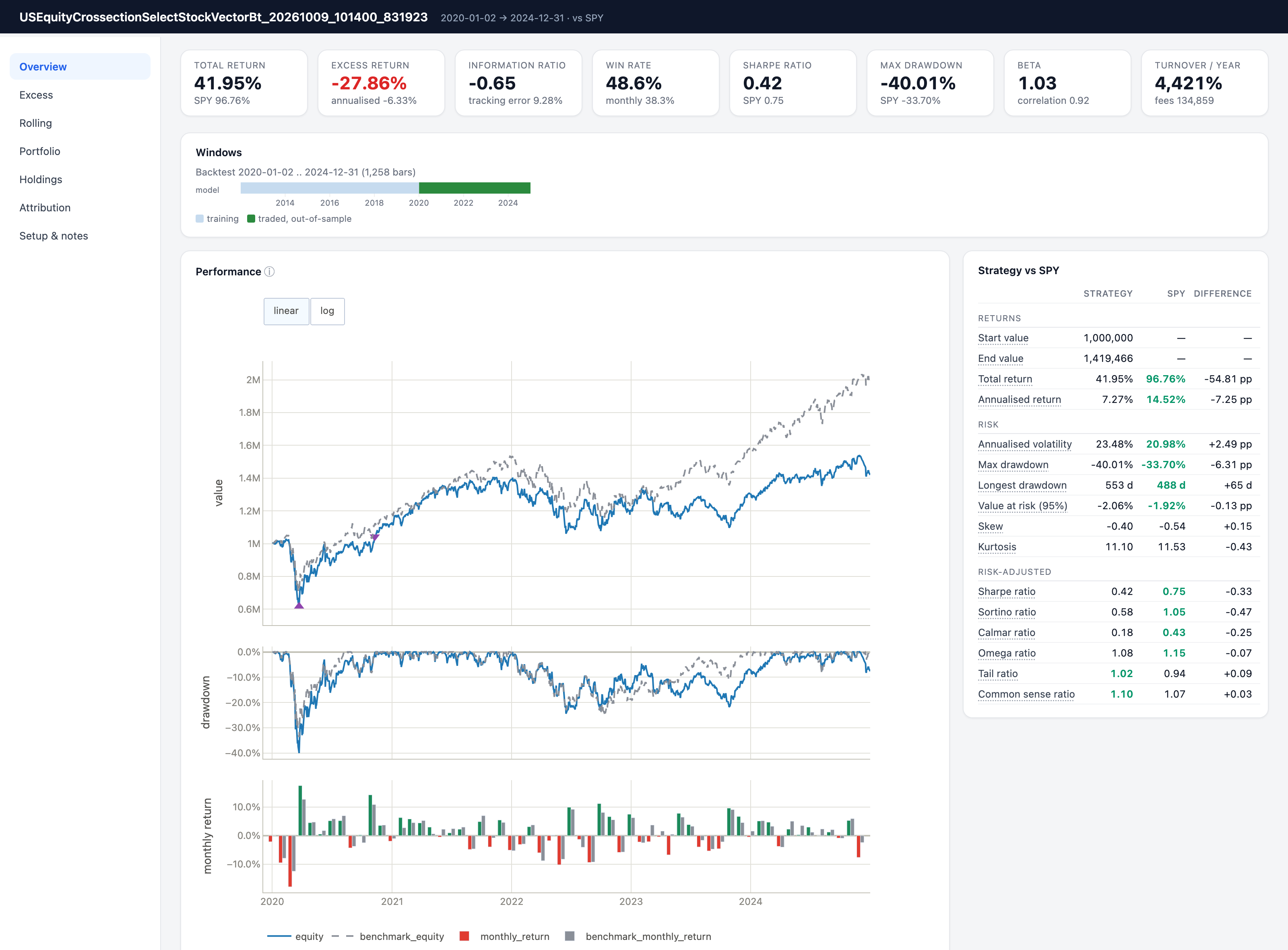
Overview: a timeline of the training and backtest windows, in-sample against out-of-sample when the run has an in-sample part, and the Performance chart (NAV, drawdown, monthly returns) beside the strategy-against-benchmark table.
Excess (with a benchmark): the cumulative excess return, log or arithmetic, and the excess drawdown.
Rolling: one-year excess return, information ratio and beta, or return, volatility and Sharpe ratio without a benchmark.
Portfolio: turnover, the number of holdings and the exposures per rebalance, beside the trading table (fees, orders, rejected orders, construction failures and events).
Holdings: which positions made the return, by size; then day by day each symbol’s target weight, holding and period return, with navigation, sorting, filtering and a CSV export.
Attribution and Factor attribution: the decompositions above.
Setup & notes: the settings no table shows, and the caveats.

When the run has an in-sample part, the headline numbers and main tables are out-of-sample and every chart shades the in-sample range. The page loads plotly.js from a CDN, so viewing it needs network access.

Tracking#

To send a backtest to an experiment tracker, set the config’s tracker, as for a model. The default NullTracker sends nothing. Each run opens one tracking run in the project <ClassName>_backtest (or the tracker’s project), named after the run directory, with the metric blocks in its summary as whole/<metric> and so on, and report.html attached. The run opens before the backtest, so a backtest that raises is recorded as failed.

>>> backtester.config.tracker
NullTracker(project=None)
>>> from quantlab.tracking.wandb import WandbTracker
>>> tracked = USEquityCrossectionSelectStockVectorBt(dataclasses.replace(
...     backtester.config, tracker=WandbTracker(project="momentum_backtests", mode="offline")
... )).run()
>>> BacktestRun.open(tracked.run_dir).rebuild("tracker")
WandbTracker(project='momentum_backtests', entity=None, mode='offline')

The run directory#

Each run writes a new directory {ClassName}_{timestamp} under output_dir. Files go to a hidden staging directory that is renamed into place once every file is written, so output_dir only holds complete runs, and an existing directory is never overwritten. A run directory is read through BacktestRun (or quantlab.runs.directory.open_run(), which opens any run directory); only the run layer names its files. What a run holds:

`BacktestRun`	Content
`kind`, `window`	`"run"`, `"run_cv"`, `"run_weights"` or `"fold"`; the first and last bar simulated.
`market`, `execution`, `rebalance_periods`	The fill and valuation columns, the sizing basis, fees and slippage, the bars between rebalances.
`weights()`, `equity()`, `holdings()`	The target weights with the rebalance record; the portfolio value and returns (and the benchmark’s); the simulated holdings, each symbol’s value over the book’s at every close.
`metrics()`, `settlements()`	The metric blocks; the delisting settlements.
`predictions()`	The predictions the rule read, with their label specs (`None` for `run_weights()`).
`trained_run()`	The trained unit the backtest used.
`data_fingerprint`, `code`	What the run read, by component path, and the code it ran.
`folds`	A `run_cv()` run’s folds.
`report()`, `factor_attribution()`	The HTML report; the per-bar factor attribution.
`rebuild(field)`, `rebuild_backtester()`	The component a config field holds; the backtester itself.

>>> run.market
Market(fill_price_column='adjOpen', valuation_price_column='adjClose')
>>> run.execution
ExecutionSettings(sizing_basis='fill', fees=0.0005, slippage=0.0005)
>>> sorted(run.data_fingerprint), run.trained_run().kind
(['model.factors.0.dataset', 'price_dataset'], 'model')
>>> sorted(run.metrics()) == sorted(result.metrics), run.metrics()["out_of_sample_ranges"]
(True, [['2024-02-26', '2024-03-22']])
>>> [spec.name for spec in run.predictions().labels], sorted(run.equity().data_vars)
(['open_ret_1'], ['returns', 'value'])

A dataset held in memory (FrameDataset) has no store, so the run keeps a copy of its panel and the recipe names it relative to the run directory, which can then be moved. All JSON files are strict JSON: NaN and infinities are written as null.

Rebuild a run#

The recipe names every class by its dotted import path, so rebuild_backtester() builds the same backtester, price dataset and model again, and run() repeats the backtest into a new directory:

>>> run = BacktestRun.open(result.run_dir)
>>> run.rebuild("constructor")
TopNConstructor(direction='long_only', top_n=2, score_label=None)
>>> again = run.rebuild_backtester().run()
>>> again.metrics["whole"] == result.metrics["whole"], again.run_dir == result.run_dir
(True, False)

Keyword arguments replace config fields by name, so a recorded run is re-run as a variant; a name that is no config field is refused:

>>> run.rebuild_backtester(rebalance_periods=10).config.rebalance_periods
10

The classes must be importable: a class defined in a script is named __main__.X and cannot be found from another process, so datasets, factors, models and backtesters belong in modules. A recipe with a missing field is refused rather than filled from today’s defaults, which may differ from the ones the run used. A train-mode run retrains when rebuilt as it is; to replay the same model, load the unit it trained:

>>> trained_run = BacktestRun.open(trained.run_dir)
>>> replayed_train = trained_run.rebuild_backtester(
...     model_mode="load", checkpoint=str(trained_run.trained_run().checkpoint)
... ).run()
>>> bool((replayed_train.weights["weight"].fillna(0) == trained.weights["weight"].fillna(0)).all())
True

A run_weights() run is replayed from the weights it saved: pass its weights() to run_weights() on the rebuilt backtester.

Data can change under a stored run: stores are appended to, and adjusted prices are restated after splits and dividends. Every read a component makes is recorded with a digest of the values, keyed by its component path. A rebuilt backtester compares its reads with the recorded ones and logs a warning for each difference, naming what changed (the variables whose values changed, a different range, added or missing variables). A rebuild also warns when a component’s module or a library version changed. Neither refuses to run, since a backtest on updated data is often what you want.

The approximate backtest#

A backtest run decides one bar at a time, replays holdings under the execution rules and writes a directory: too slow to sweep a rule’s parameters or compare many models. The approximate backtest (ApproximateBacktest; for US equities USEquityApproximateBacktest) decides every rebalance of a prediction panel at once and simulates the window as array operations. Build it once over a price dataset and a window, then run it on as many (predictions, rule) pairs as you like; the prices are read once and nothing is written. Use it to choose, and confirm the choice with run(), which takes the same rule config unchanged.

Continuing the first session, the run’s recorded predictions go to an approximate backtest over the same window; cost stands for fees plus slippage:

>>> from quantlab.backtest.config import ApproximateBacktestConfig
>>> from quantlab.backtest.predefined.us_equity import USEquityApproximateBacktest
>>> approximate = USEquityApproximateBacktest(ApproximateBacktestConfig(
...     price_dataset=prices_of(cfg),
...     start_date="2024-02-12",
...     end_date="2024-03-22",
...     rebalance_periods=5,
...     cost=0.001,
... ))
>>> predictions = run.predictions()
>>> account = approximate.run(predictions, TopNConstructor(TopNConfig(direction="long_only", top_n=2)))
>>> round(account.metrics["whole"]["Total Return [%]"], 2), round(run.metrics()["whole"]["Total Return [%]"], 2)
(-5.92, -5.87)
>>> account.weights["weight"].fillna(9).equals(result.weights["weight"].fillna(9))
True
>>> for top_n in (1, 2, 3):
...     swept = approximate.run(predictions, TopNConstructor(TopNConfig(direction="long_only", top_n=top_n)))
...     print(top_n, round(swept.metrics["whole"]["Sharpe Ratio"], 2), round(swept.metrics["whole"]["Turnover per Rebalance [%]"], 1))
1 -6.22 150.0
2 -2.36 134.1
3 -1.42 84.4
>>> round(backtester.run_weights(account.weights).metrics["whole"]["Total Return [%]"], 2)
-5.87

The weights are the run’s, with its rebalance record, so run_weights takes them as they are and gives the run back; the 0.05-point gap in total return is FFF’s delisting.

What it keeps and what it gives up#

It keeps the rebalance schedule, the t+1 fill at the open, holdings marked at the close and drifting between fills, tradability judged at the decision bar, and the statistics, computed by the same functions as a run’s metrics. It gives up, each a source of gap from run():

Rejected orders: a missing fill price falls back to the previous close.
Locked positions: a held symbol that cannot trade is sold at the next rebalance at the price it stopped at.
Delisting settlements: a delisted holding stays at its last valuation until a rebalance sells it.
The cash cap: a run cuts a fill’s last buys to the cash the fees leave; the approximation does not, so with fees the holdings differ by about cost times turnover.
Order mechanics: fees and slippage are one cost on traded weight; min_trade is not modelled.
The name-count cap: with max_names the names are a local optimum, where run() solves the mixed-integer program exactly.

On synthetic stores without these events, TopNConstructor gives the run’s weights exactly and mean-variance within 2e-7 (L1) of a tightly solved run. On a store with delistings, a listing, a halt and missing fill prices, the value stays within 2.3e-2 over a 68-bar window. On real data the gap grows with how often held names halt, delist or miss a fill price.

Rules#

It runs the shipped rules, each through its own implementation chosen by the rule’s exact class (see Portfolio construction for the supported fields). A custom rule, or a subclass of a shipped one, is refused before any data is read:

>>> from quantlab.portfolio.config import TopNConfig
>>> from quantlab.portfolio.predefined.top_n import TopNConstructor
>>> class EqualWeightTopN(TopNConstructor):
...     pass
>>> approximate.run(predictions, EqualWeightTopN(TopNConfig(direction="long_only", top_n=2)))
Traceback (most recent call last):
ValueError: USEquityApproximateBacktest cannot run EqualWeightTopN: EqualWeightTopN has no approximate implementation: the approximate backtest runs TopNConstructor, TopkDropoutConstructor, MeanVarianceOptimizer, ActiveRiskOptimizer, BlackLittermanOptimizer, as those exact classes; backtest it with a backtest run

The window is cut into chunks of chunk_bars bars (default 63), decided in time order, which bounds memory without changing the result. A rule whose decision reads the holdings (a turnover penalty, candidate_top_k, TopkDropout) solves its bars forward, each once from the previous bar’s book; otherwise the bars are solved at once. A mean-variance bar has converged when its residual is at most tolerance (default 1e-5) times its starting gradient’s largest entry; after max_iterations a warning names the bars and converged is False.

>>> from quantlab.portfolio.config import (
...     GrinoldExpectedReturnConfig, LedoitWolfEstimatorConfig, MeanVarianceConfig,
... )
>>> from quantlab.portfolio.predefined.expected_return import GrinoldExpectedReturn
>>> from quantlab.portfolio.predefined.ledoit_wolf import LedoitWolfEstimator
>>> from quantlab.portfolio.predefined.mean_variance import MeanVarianceOptimizer
>>> for penalty in (0.0, 0.002):
...     rule = MeanVarianceOptimizer(MeanVarianceConfig(
...         expected_return_label="open_ret_1",
...         covariance=LedoitWolfEstimator(LedoitWolfEstimatorConfig(lookback_bars=10)),
...         expected_return=GrinoldExpectedReturn(GrinoldExpectedReturnConfig(ic=0.05)), risk_aversion=5.0, weight_cap=0.5, turnover_penalty=penalty,
...     ))
...     solved = approximate.run(predictions, rule)
...     print(penalty, round(solved.metrics["whole"]["Turnover per Rebalance [%]"], 1), solved.metrics["iterations"]["max"])
0.0 118.2 6
0.002 34.6 5

The account#

run returns an ApproximateAccount: the account record a run’s metrics are built from, the value with and without costs, the weights in a run’s format (so run_weights takes them), the equal-weighted universe, and metrics with a run’s whole, execution and attribution blocks plus the solver’s iterations and converged. With benchmark_dataset the metrics gain a run’s benchmark and relative blocks:

approximate = USEquityApproximateBacktest(dataclasses.replace(approximate.config, benchmark_dataset=spy))
account = approximate.run(predictions, rule)
account.metrics["relative"]["whole"]["Information Ratio"]

Metrics and reports outside a backtester#

An executor that trades elsewhere, such as an event-driven backtest or a live account, can report in quantlab’s format without the backtester:

quantlab.runs.backtest_stats computes the return, relative, win-rate, turnover and round-trip rows of the metrics from plain arrays (numpy, pandas and xarray only).
quantlab.runs.run_metrics.run_metrics() assembles the metric blocks from an AccountRecord, what one account did over its bars; BaseBacktester.account(simulation) returns a simulation’s record.
quantlab.runs.backtest_report.write_backtest_report() writes report.html from an account record, with ReportExtras for what only some runs have.
quantlab.execution.rules holds the execution rules the engine fills a bar by (rejection without a fill price, delisting settlement, sizing basis, sells before buys, buys capped by the cash left, fees and slippage). replay returns the shares and cash a weight panel leaves after every bar; ExecutionBook holds the same book one bar at a time.

>>> import numpy as np
>>> from quantlab.execution.rules import ExecutionSettings, replay
>>> prices = np.array([[10.0], [10.0]])
>>> book = replay(
...     np.array([[1.0], [np.nan]]), prices, prices, np.zeros((2, 1), dtype=bool),
...     ExecutionSettings(fees=0.01),
... )
>>> round(float(book.shares[1, 0]), 10), float(book.cash[1])
(0.099009901, 0.0)

The whole book in one stock at 10 with a 1% fee costs more than the cash, so the buy is cut until cost and fee equal it.

Extending#

A new market is a MarketSpec with its own price columns and annualisation; a new selection rule is usually a portfolio construction rule. To write either, or a new engine, see Extending quantlab.

An event-driven engine is reserved but not implemented.